
Intro to Rubin Catalog Operations#
In this tutorial, we will:
explore the basics of column discovery
work with an individual lightcurve
learn about the LSDB lightcurve plotting utilities
apply common filtering operations
calculate basic aggregation statistics
Introduction#
This tutorial showcases a handful of basic LSDB operations that should be useful when working with Rubin (DP1) data. These operations are likely to be used regardless of science case, and the particular examples in this tutorial should allow you to understand how to use these operations in other ways. For example, while we filter by photometric band in one of the example below, that filter can easily be modified to filter by a quality flag in the data.
1. Install and import required packages#
Here we introduce lsdb-rubin, a package developed to support LSDB operations on Rubin data, on the RSP (Rubin Science Platform).
Rubin provides multi-band photometry in ugrizy, and HATS-ified Rubin data will serve this in nested dataframes.
[1]:
# Uncomment to install lsdb
# %pip install --quiet -U lsdb-rubin
[2]:
from upath import UPath
import lsdb
from lsdb import ConeSearch
from lsdb_rubin.plot_light_curve import plot_light_curve
import matplotlib.pyplot as plt
2. Loading Data#
The details of loading Rubin data are discussed in How to Access Data, so we’ll just provide a starter codeblock below:
[3]:
base_path = UPath("/rubin/lsdb_data")
object_collection = lsdb.open_catalog(base_path / "object_collection")

# Cone search on ECDFS (Extended Chandra Deep Field South)
object_collection = lsdb.open_catalog(
    base_path / "dia_object_collection",
    search_filter=ConeSearch(ra=52.838, dec=-28.279, radius_arcsec=5000),
)
object_collection
[3]:
| dec | diaObjectId | nDiaSources | ra | radecMjdTai | tract | diaObjectForcedSource | diaSource | |
|---|---|---|---|---|---|---|---|---|
| npartitions=42 | ||||||||
| Order: 10, Pixel: 9198847 | double[pyarrow] | int64[pyarrow] | int64[pyarrow] | double[pyarrow] | double[pyarrow] | int64[pyarrow] | nested<band: [string], coord_dec: [double], co... | nested<band: [string], centroid_flag: [bool], ... |
| Order: 6, Pixel: 35933 | ... | ... | ... | ... | ... | ... | ... | ... |
| ... | ... | ... | ... | ... | ... | ... | ... | ... |
| Order: 7, Pixel: 143825 | ... | ... | ... | ... | ... | ... | ... | ... |
| Order: 6, Pixel: 35957 | ... | ... | ... | ... | ... | ... | ... | ... |
As mentioned beneath the catalog dataframe, the view above is a “lazy” view of the data. Often, it’s nice to preview the first few rows to better understand the contents of the dataset:
[4]:
object_collection.head(5)
[4]:
| dec | diaObjectId | nDiaSources | ra | radecMjdTai | tract | diaObjectForcedSource | diaSource | ||||||||||||||||||||||||||
|---|---|---|---|---|---|---|---|---|---|---|---|---|---|---|---|---|---|---|---|---|---|---|---|---|---|---|---|---|---|---|---|---|---|
| 2528559836917790087 | -28.694949 | 609787430777651220 | 1 | 53.446451 | 60632.084896 | 4849 |
|
|
|||||||||||||||||||||||||
| 2528559862939733327 | -28.688946 | 609787430777651219 | 1 | 53.439723 | 60632.084896 | 4849 |
|
|
|||||||||||||||||||||||||
| 2528559881657338699 | -28.688324 | 609787362058174465 | 1 | 53.459674 | 60632.084896 | 4849 |
|
|
|||||||||||||||||||||||||
| 2528560064243227454 | -28.648182 | 609788117972418767 | 1 | 53.429821 | 60632.073989 | 4849 |
|
|
|||||||||||||||||||||||||
| 2528606911361164817 | -28.630057 | 609788049252941917 | 1 | 53.505678 | 60632.084896 | 4849 |
|
|
3. Viewing Available Columns#
The schema browser provides the most information regarding available (DP1) columns, there is also a handful of properties useful for quick column discovery within the LSDB API. First, all_columns gives a view of all available columns in the HATS catalog, even if only a handful of columns were selected on load:
[5]:
object_collection.all_columns
[5]:
['ra',
 'dec',
 'nDiaSources',
 'radecMjdTai',
 'g_psfFluxLinearSlope',
 'g_psfFluxLinearIntercept',
 'g_psfFluxMAD',
 'g_psfFluxMaxSlope',
 'g_psfFluxErrMean',
 'g_psfFluxMean',
 'g_psfFluxMeanErr',
 'g_psfFluxNdata',
 'g_scienceFluxMean',
 'g_scienceFluxMeanErr',
 'g_psfFluxMin',
 'g_psfFluxMax',
 'g_psfFluxPercentile05',
 'g_psfFluxPercentile25',
 'g_psfFluxPercentile50',
 'g_psfFluxPercentile75',
 'g_psfFluxPercentile95',
 'g_psfFluxSigma',
 'g_scienceFluxSigma',
 'g_psfFluxSkew',
 'g_psfFluxChi2',
 'g_psfFluxStetsonJ',
 'r_psfFluxLinearSlope',
 'r_psfFluxLinearIntercept',
 'r_psfFluxMAD',
 'r_psfFluxMaxSlope',
 'r_psfFluxErrMean',
 'r_psfFluxMean',
 'r_psfFluxMeanErr',
 'r_psfFluxNdata',
 'r_scienceFluxMean',
 'r_scienceFluxMeanErr',
 'r_psfFluxMin',
 'r_psfFluxMax',
 'r_psfFluxPercentile05',
 'r_psfFluxPercentile25',
 'r_psfFluxPercentile50',
 'r_psfFluxPercentile75',
 'r_psfFluxPercentile95',
 'r_psfFluxSigma',
 'r_scienceFluxSigma',
 'r_psfFluxSkew',
 'r_psfFluxChi2',
 'r_psfFluxStetsonJ',
 'u_psfFluxLinearSlope',
 'u_psfFluxLinearIntercept',
 'u_psfFluxMAD',
 'u_psfFluxMaxSlope',
 'u_psfFluxErrMean',
 'u_psfFluxMean',
 'u_psfFluxMeanErr',
 'u_psfFluxNdata',
 'u_scienceFluxMean',
 'u_scienceFluxMeanErr',
 'u_psfFluxMin',
 'u_psfFluxMax',
 'u_psfFluxPercentile05',
 'u_psfFluxPercentile25',
 'u_psfFluxPercentile50',
 'u_psfFluxPercentile75',
 'u_psfFluxPercentile95',
 'u_psfFluxSigma',
 'u_scienceFluxSigma',
 'u_psfFluxSkew',
 'u_psfFluxChi2',
 'u_psfFluxStetsonJ',
 'i_psfFluxLinearSlope',
 'i_psfFluxLinearIntercept',
 'i_psfFluxMAD',
 'i_psfFluxMaxSlope',
 'i_psfFluxErrMean',
 'i_psfFluxMean',
 'i_psfFluxMeanErr',
 'i_psfFluxNdata',
 'i_scienceFluxMean',
 'i_scienceFluxMeanErr',
 'i_psfFluxMin',
 'i_psfFluxMax',
 'i_psfFluxPercentile05',
 'i_psfFluxPercentile25',
 'i_psfFluxPercentile50',
 'i_psfFluxPercentile75',
 'i_psfFluxPercentile95',
 'i_psfFluxSigma',
 'i_scienceFluxSigma',
 'i_psfFluxSkew',
 'i_psfFluxChi2',
 'i_psfFluxStetsonJ',
 'z_psfFluxLinearSlope',
 'z_psfFluxLinearIntercept',
 'z_psfFluxMAD',
 'z_psfFluxMaxSlope',
 'z_psfFluxErrMean',
 'z_psfFluxMean',
 'z_psfFluxMeanErr',
 'z_psfFluxNdata',
 'z_scienceFluxMean',
 'z_scienceFluxMeanErr',
 'z_psfFluxMin',
 'z_psfFluxMax',
 'z_psfFluxPercentile05',
 'z_psfFluxPercentile25',
 'z_psfFluxPercentile50',
 'z_psfFluxPercentile75',
 'z_psfFluxPercentile95',
 'z_psfFluxSigma',
 'z_scienceFluxSigma',
 'z_psfFluxSkew',
 'z_psfFluxChi2',
 'z_psfFluxStetsonJ',
 'y_psfFluxLinearSlope',
 'y_psfFluxLinearIntercept',
 'y_psfFluxMAD',
 'y_psfFluxMaxSlope',
 'y_psfFluxErrMean',
 'y_psfFluxMean',
 'y_psfFluxMeanErr',
 'y_psfFluxNdata',
 'y_scienceFluxMean',
 'y_scienceFluxMeanErr',
 'y_psfFluxMin',
 'y_psfFluxMax',
 'y_psfFluxPercentile05',
 'y_psfFluxPercentile25',
 'y_psfFluxPercentile50',
 'y_psfFluxPercentile75',
 'y_psfFluxPercentile95',
 'y_psfFluxSigma',
 'y_scienceFluxSigma',
 'y_psfFluxSkew',
 'y_psfFluxChi2',
 'y_psfFluxStetsonJ',
 'diaObjectId',
 'tract',
 'diaSource',
 'diaObjectForcedSource']
Any nested columns (see Understanding the NestedFrame for an explanation on what these are) will have their own sets of sub-columns as well, we can first identify any nested columns programmatically using the nested_columns property:
[6]:
object_collection.nested_columns
[6]:
['diaObjectForcedSource', 'diaSource']
To view the available sub-columns, we use the nest accessor for one of the nested columns:
[7]:
object_collection["diaObjectForcedSource"].columns
[7]:
['band',
 'coord_dec',
 'coord_ra',
 'diff_PixelFlags_nodataCenter',
 'forcedSourceOnDiaObjectId',
 'invalidPsfFlag',
 'midpointMjdTai',
 'pixelFlags_bad',
 'pixelFlags_cr',
 'pixelFlags_crCenter',
 'pixelFlags_edge',
 'pixelFlags_interpolated',
 'pixelFlags_interpolatedCenter',
 'pixelFlags_nodata',
 'pixelFlags_saturated',
 'pixelFlags_saturatedCenter',
 'pixelFlags_suspect',
 'pixelFlags_suspectCenter',
 'psfDiffFlux',
 'psfDiffFlux_flag',
 'psfDiffFluxErr',
 'psfFlux',
 'psfFlux_flag',
 'psfFluxErr',
 'psfMag',
 'psfMagErr',
 'visit']
4. Viewing a Single Lightcurve#
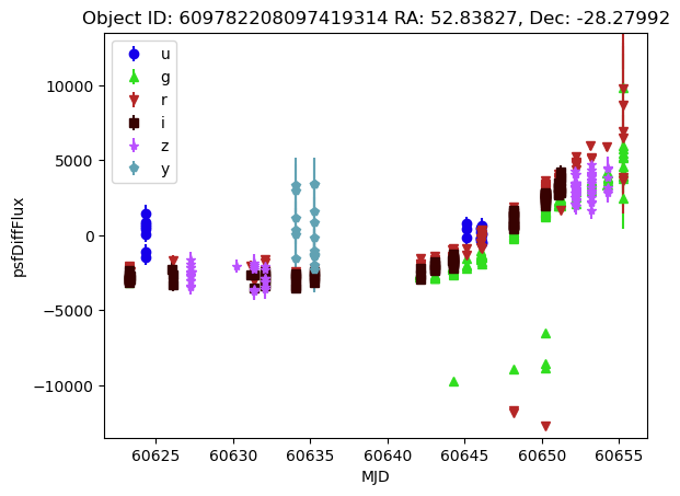
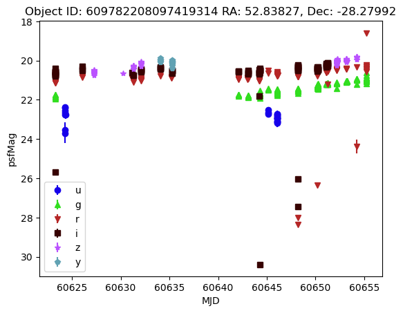
You can find more information on the plotting utility plot_light_curve at the lsdb-rubin readthedocs.
The lightcurve has an outlier, so we can use the plt.gca() method to get the current matplotlib axis and effectively crop out the outliers.
Selecting a single lightcurve is most effectively done via the id_search function, in this case we have a particular “diaObjectId” in mind:
[8]:
objectid = 609782208097419314
single_id = object_collection.id_search(values={"diaObjectId": objectid}).compute()
single_id
Searching for diaObjectId=609782208097419314
[8]:
| dec | diaObjectId | nDiaSources | ra | radecMjdTai | tract | diaObjectForcedSource | diaSource | |||||||||||||||||||||||||||||||
|---|---|---|---|---|---|---|---|---|---|---|---|---|---|---|---|---|---|---|---|---|---|---|---|---|---|---|---|---|---|---|---|---|---|---|---|---|---|---|
| 2528690302717534293 | -28.279918 | 609782208097419314 | 371 | 52.838269 | 60655.249976 | 4848 |
|
|
[9]:
plot_light_curve(
    single_id.iloc[0]["diaObjectForcedSource"],
    flux_field="psfDiffFlux",
    title=f'Object ID: {single_id["diaObjectId"].values[0]} RA: {single_id["ra"].values[0]:.5f}, Dec: {single_id["dec"].values[0]:.5f}',
)
plt.gca().set_ylim([-13_500, 13_500])
[9]:
(-13500.0, 13500.0)
[10]:
plot_light_curve(
    single_id.iloc[0]["diaObjectForcedSource"],
    mag_field="psfMag",
    title=f'Object ID: {single_id["diaObjectId"].values[0]} RA: {single_id["ra"].values[0]:.5f}, Dec: {single_id["dec"].values[0]:.5f}',
)
5. Common Filtering Operations#
5.1. Filtering by Number of Sources#
Provided the Source table(s) haven’t been modified by any filtering operations, the “nDiaSources” column is directly provided and allows for easy filtering based on lightcurve length. Note that “nDiaSources” is just a static column that maps to the unmodified lengths of DiaSources, once the number of DiaSources is modified then the value in this column will be out of date.
[11]:
oc_long_lcs = object_collection.query("nDiaSources > 10")
oc_long_lcs.head(5)
[11]:
| dec | diaObjectId | nDiaSources | ra | radecMjdTai | tract | diaObjectForcedSource | diaSource | |||||||||||||||||||||||||||||||
|---|---|---|---|---|---|---|---|---|---|---|---|---|---|---|---|---|---|---|---|---|---|---|---|---|---|---|---|---|---|---|---|---|---|---|---|---|---|---|
| 2528607275717728666 | -28.583791 | 609788049252941847 | 12 | 53.489935 | 60651.220877 | 4849 |
|
|
||||||||||||||||||||||||||||||
| 2528607345986705737 | -28.559039 | 609788049252941850 | 12 | 53.512649 | 60651.220877 | 4849 |
|
|
||||||||||||||||||||||||||||||
| 2528608083060939470 | -28.541942 | 609788049252941840 | 13 | 53.556345 | 60652.209345 | 4849 |
|
|
||||||||||||||||||||||||||||||
| 2528608127600158337 | -28.532665 | 609788049252941831 | 13 | 53.574546 | 60652.209345 | 4849 |
|
|
||||||||||||||||||||||||||||||
| 2528608365089811280 | -28.505685 | 609788736447709250 | 11 | 53.586313 | 60651.101656 | 4849 |
|
|
5.2. Filtering by Photometric Band#
Another common operation is to filter by band, which can done similarly to above, but using sub-column queries:
[12]:
oc_long_lcs_g = oc_long_lcs.query("diaObjectForcedSource.band == 'g'")
oc_long_lcs_g.head(5)
[12]:
| dec | diaObjectId | nDiaSources | ra | radecMjdTai | tract | diaObjectForcedSource | diaSource | |||||||||||||||||||||||||||||||
|---|---|---|---|---|---|---|---|---|---|---|---|---|---|---|---|---|---|---|---|---|---|---|---|---|---|---|---|---|---|---|---|---|---|---|---|---|---|---|
| 2528607275717728666 | -28.583791 | 609788049252941847 | 12 | 53.489935 | 60651.220877 | 4849 |
|
|
||||||||||||||||||||||||||||||
| 2528607345986705737 | -28.559039 | 609788049252941850 | 12 | 53.512649 | 60651.220877 | 4849 |
|
|
||||||||||||||||||||||||||||||
| 2528608083060939470 | -28.541942 | 609788049252941840 | 13 | 53.556345 | 60652.209345 | 4849 |
|
|
||||||||||||||||||||||||||||||
| 2528608127600158337 | -28.532665 | 609788049252941831 | 13 | 53.574546 | 60652.209345 | 4849 | None |
|
||||||||||||||||||||||||||||||
| 2528608365089811280 | -28.505685 | 609788736447709250 | 11 | 53.586313 | 60651.101656 | 4849 |
|
|
Note: Filtering operations on “diaObjectForcedSource” are not propagated to “diaSource”. Any filtering operations on “diaSource” should be applied in addition to any operations done on “diaObjectForcedSource”.
5.3. Filtering Empty Lightcurves#
Sometimes, filters on lightcurves may throw out all observations for certain objects, leading to empty lightcurves as seen for one of the objects above. In this case, we can filter objects with empty lightcurves using dropna:
[13]:
oc_long_lcs_g = oc_long_lcs_g.map_partitions(lambda df: df.dropna(subset=["diaObjectForcedSource"]))
oc_long_lcs_g.head(5)
[13]:
| dec | diaObjectId | nDiaSources | ra | radecMjdTai | tract | diaObjectForcedSource | diaSource | |||||||||||||||||||||||||||||||
|---|---|---|---|---|---|---|---|---|---|---|---|---|---|---|---|---|---|---|---|---|---|---|---|---|---|---|---|---|---|---|---|---|---|---|---|---|---|---|
| 2528607275717728666 | -28.583791 | 609788049252941847 | 12 | 53.489935 | 60651.220877 | 4849 |
|
|
||||||||||||||||||||||||||||||
| 2528607345986705737 | -28.559039 | 609788049252941850 | 12 | 53.512649 | 60651.220877 | 4849 |
|
|
||||||||||||||||||||||||||||||
| 2528608083060939470 | -28.541942 | 609788049252941840 | 13 | 53.556345 | 60652.209345 | 4849 |
|
|
||||||||||||||||||||||||||||||
| 2528608365089811280 | -28.505685 | 609788736447709250 | 11 | 53.586313 | 60651.101656 | 4849 |
|
|
||||||||||||||||||||||||||||||
| 2528608386523759343 | -28.494832 | 609788736447709234 | 19 | 53.584151 | 60651.101656 | 4849 |
|
|
6. Calculating Basic Statistics#
While Rubin DP1 data has many statistics pre-computed in object table column, custom computation of statistics remains broadly useful.
Simple aggregrations can be applied via the map_rows function, where below we define a very simple mean magnitude function and pass it along to each row, selecting the “psfMag” sub-column of “diaObjectForcedSource” to compute the mean of for each object.
[14]:
import numpy as np


def mean_mag(row):
    return {"mean_psfMag": np.mean(row["diaObjectForcedSource.psfMag"])}


# meta defines the expected structure of the result
# append_columns adds the result as a column to the original catalog
oc_mean_mags_g = oc_long_lcs_g.map_rows(
    mean_mag, columns=["diaObjectForcedSource.psfMag"], meta={"mean_psfMag": np.float64}, append_columns=True
)
oc_mean_mags_g.head(10)[["mean_psfMag"]]
[14]:
| mean_psfMag | |
|---|---|
| _healpix_29 | |
| 2528607275717728666 | 19.411814 |
| 2528607345986705737 | 19.042889 |
| 2528608083060939470 | 17.257166 |
| 2528608365089811280 | 17.539051 |
| 2528608386523759343 | 19.579895 |
| 2528611470051636305 | 19.204950 |
| 2528611708541527859 | 19.087742 |
| 2528611724254005370 | 18.638960 |
| 2528652384125757089 | 17.412634 |
| 2528653248294272515 | 18.371521 |
10 rows × 1 columns
In this example, we needed to define the dask “meta”, see here for a more dedicated discussion on meta.
About#
Author(s): Doug Branton
Last updated on: 11 May 2026
If you use lsdb for published research, please cite following instructions.
[ ]: