Large Crossmatches with EDP2

Large Crossmatches with EDP2#

In this notebook we’ll show how to:

Load the HATS-formatted version of DP2 on the Rubin Science Platform (RSP)
Load an external HATS catalog
Apply column-based filtering on catalogs
Perform large crossmatches between DP2 and other catalogs
Demonstrate how to use Catalog streaming to overcome significant data volume
Plot some resulting lightcurves

[1]:

import lsdb
from upath import UPath
from dask.distributed import Client
from lsdb.streams import CatalogStream
import pandas as pd
import matplotlib.pyplot as plt

[2]:

import logging

logging.getLogger().setLevel(logging.WARNING)
logging.getLogger("distributed").setLevel(logging.WARNING)

[3]:

plt.rcParams.update(
    {
        "axes.titlesize": 16,
        "axes.labelsize": 15,
        "xtick.labelsize": 13,
        "ytick.labelsize": 13,
        "legend.fontsize": 13,
        "figure.titlesize": 18,
    }
)

Load Data Preview 2#

We begin by loading in DP2, specifying just ra and dec columns to have the lightest weight catalog possible. In practice, trimming down columns to only the subset you’ll need for analysis can greatly help in avoiding memory-related issues during computation.

Tip: It’s fine to load them all lazily at first and then trim down later once you’ve solidified a workflow.

[4]:

dp2_path = UPath("/rubin/lsdb_data/object_collection")

dp2 = lsdb.open_catalog(dp2_path, columns=["coord_ra", "coord_dec"])
dp2

[4]:

lsdb Catalog object_lc:

	coord_ra	coord_dec
npartitions=8840
Order: 8, Pixel: 10240	double[pyarrow]	double[pyarrow]
...	...	...
Order: 5, Pixel: 12283	...	...
Order: 5, Pixel: 12284	...	...

2 out of 1261 available columns in the catalog have been loaded lazily, meaning no data has been read, only the catalog schema

This catalog has an estimated size of 18.9 GB

Load another Catalog - Gaia DR3#

We’ll now load Gaia remotely as a second catalog for future crossmatching. Again, we’re limiting our column loading to only columns we’ll need.

Many public catalogs are available to load directly with LSDB — you can browse them at data.lsdb.io.

[5]:

# Open from a remote s3 bucket
gaia = lsdb.open_catalog(
    "s3://stpubdata/gaia/gaia_dr3/public/hats",
    columns=[
        "ra",
        "dec",
        "parallax",
        "parallax_over_error",
        "teff_gspphot",
        "logg_gspphot",
        "classprob_dsc_combmod_star",
    ],
)
gaia

[5]:

lsdb Catalog gaia:

	ra	dec	parallax	parallax_over_error	teff_gspphot	logg_gspphot	classprob_dsc_combmod_star
npartitions=2016
Order: 2, Pixel: 0	double[pyarrow]	double[pyarrow]	double[pyarrow]	float[pyarrow]	float[pyarrow]	float[pyarrow]	float[pyarrow]
...	...	...	...	...	...	...	...
Order: 3, Pixel: 766	...	...	...	...	...	...	...
Order: 3, Pixel: 767	...	...	...	...	...	...	...

7 out of 152 available columns in the catalog have been loaded lazily, meaning no data has been read, only the catalog schema

This catalog has an estimated size of 87.0 GB

Query Gaia: Filtering for FGK Stars#

Catalog.query allows us to apply filters based on column values, in this case we’ll apply a set of cuts to select for FGK Stars.

[6]:

gaia_filtered = gaia.query("parallax > 0 and parallax_over_error > 5 and \
    teff_gspphot > 5380 and teff_gspphot < 7220 and logg_gspphot > 4.5 \
    and logg_gspphot < 4.72 and classprob_dsc_combmod_star > 0.5")

Perform a Crossmatch#

Now we’re ready to crossmatch DP2 and our filtered Gaia DR3.

[7]:

xmatch = dp2.crossmatch(gaia_filtered, suffix_method="overlapping_columns")
xmatch

[7]:

lsdb Catalog object_lc_x_gaia:

	coord_ra	coord_dec	ra	dec	parallax	parallax_over_error	teff_gspphot	logg_gspphot	classprob_dsc_combmod_star	_dist_arcsec
npartitions=9139
Order: 8, Pixel: 10240	double[pyarrow]	double[pyarrow]	double[pyarrow]	double[pyarrow]	double[pyarrow]	float[pyarrow]	float[pyarrow]	float[pyarrow]	float[pyarrow]	double[pyarrow]
...	...	...	...	...	...	...	...	...	...	...
Order: 5, Pixel: 12283	...	...	...	...	...	...	...	...	...	...
Order: 5, Pixel: 12284	...	...	...	...	...	...	...	...	...	...

10 out of 10 available columns in the catalog have been loaded lazily, meaning no data has been read, only the catalog schema

Count the Resulting Matches#

At this point, we’re just interested in the number of matches we found, so we’ll construct a small function to apply through Catalog.map_partition which counts the number of matches in each output partition.

[8]:

# Write a simple map_partitions function to count resulting matches
def count_matches(df):
    return {"n_matches": len(df)}


matches_by_partition = xmatch.map_partitions(count_matches)

Performing Computation#

For computation, we establish a Dask Client and dictate a number of workers and memory limit per worker. The Dask client will work within it’s boundaries to perform the computation that we kick off with Catalog.compute() in parallel.

[9]:

# Define a client, and .compute() the match result
with Client(n_workers=4, threads_per_worker=1, memory_limit="4GB") as client:
    print(f"Dask dashboard: {client.dashboard_link}")
    match_df = matches_by_partition.compute()
    client.close()

Dask dashboard: https://ncaplar.nb.data-int.lsst.cloud/nb/user/ncaplar/proxy/8787/status

Finally we can check the total number of Gaia-filtered FGK stars we matched in DP2:

[10]:

print(f"Number of Matches: {match_df["n_matches"].sum()}")

Number of Matches: 548168

Including Lightcurves#

Let’s start again, but this time we’ll add the “ObjectForcedSource” column, which includes our lightcurves, with the goal of inspecting a few of them.

[11]:

dp2_lc = lsdb.open_catalog(dp2_path, columns=["coord_ra", "coord_dec", "objectForcedSource"])
dp2_lc

[11]:

lsdb Catalog object_lc:

	coord_ra	coord_dec	objectForcedSource
npartitions=8840
Order: 8, Pixel: 10240	double[pyarrow]	double[pyarrow]	nested<parentObjectId: [int64], coord_ra: [dou...
...	...	...	...
Order: 5, Pixel: 12283	...	...	...
Order: 5, Pixel: 12284	...	...	...

3 out of 1261 available columns in the catalog have been loaded lazily, meaning no data has been read, only the catalog schema

This catalog has an estimated size of 1.3 TB

A common operation is to filter lightcurve lengths, we lack a pre-existing column to tell us the lengths, so we’ll take advantage of our nested column itself to perform the filter:

[12]:

# query for lightcurves with at least 50 observations
def filter_lengths(nf):
    # define a function that applies to each dataframe partition
    return nf[nf["objectForcedSource"].len() > 50]  # nested columns have a direct len()


dp2_lc_filtered = dp2_lc.map_partitions(filter_lengths)

Now we can redo our crossmatch with Gaia:

[13]:

xmatch_lc = dp2_lc_filtered.crossmatch(gaia_filtered, suffix_method="overlapping_columns")
xmatch_lc

[13]:

lsdb Catalog object_lc_x_gaia:

	coord_ra	coord_dec	objectForcedSource	ra	dec	parallax	parallax_over_error	teff_gspphot	logg_gspphot	classprob_dsc_combmod_star	_dist_arcsec
npartitions=9139
Order: 8, Pixel: 10240	double[pyarrow]	double[pyarrow]	nested<parentObjectId: [int64], coord_ra: [dou...	double[pyarrow]	double[pyarrow]	double[pyarrow]	float[pyarrow]	float[pyarrow]	float[pyarrow]	float[pyarrow]	double[pyarrow]
...	...	...	...	...	...	...	...	...	...	...	...
Order: 5, Pixel: 12283	...	...	...	...	...	...	...	...	...	...	...
Order: 5, Pixel: 12284	...	...	...	...	...	...	...	...	...	...	...

11 out of 11 available columns in the catalog have been loaded lazily, meaning no data has been read, only the catalog schema

[14]:

# And re-initialize our counting result
def count_matches(df):
    return {"n_matches": len(df)}


matches_by_partition_lc = xmatch_lc.map_partitions(count_matches)

Dealing with Heavy Workloads - Catalog Streaming#

However, our added lightcurves add a ton of weight to the DP2 catalog. If you check the estimated catalog size when we first loaded the catalogs, you can see that DP2 was ~20GB total when loading just the “coord_ra” and “coord_dec” columns, but with “objectForcedSource” this balloons to ~1.3TB. Due to this, it’s likely that direct computation on a RSP environment (4 cores, 32GB total) will fail. We can take advantage of an alternative computation method, Catalog Streaming, in cases like this:

[15]:

%%time
match_stream = CatalogStream(xmatch_lc, partitions_per_chunk=4, shuffle=False)

chunks = []
# 16 GB workers end up being needed to perform this workflow
with Client(n_workers=1, threads_per_worker=1, memory_limit="16GB") as client:
    print(f"Dask dashboard: {client.dashboard_link}")
    print(client)
    match_iter = iter(match_stream)
    for i in range(50):
        chunks.append(next(match_iter))
    client.close()
match_df = pd.concat(chunks)
match_df

Dask dashboard: https://ncaplar.nb.data-int.lsst.cloud/nb/user/ncaplar/proxy/8787/status
<Client: 'tcp://127.0.0.1:36333' processes=1 threads=1, memory=14.90 GiB>
CPU times: user 38.9 s, sys: 3.79 s, total: 42.7 s
Wall time: 14min 28s

[15]:

coord_ra

coord_dec

objectForcedSource

ra

dec

parallax

parallax_over_error

teff_gspphot

logg_gspphot

classprob_dsc_combmod_star

_dist_arcsec

3452204825677797065

305.946264

-10.583908

parentObjectId	coord_ra	...	psfDiffFluxErr_corrected_flag	psfMagErr_corrected
0	305.946264	...	False	0.012127
+52 rows	...	...	...	...

305.946255

-10.583901

0.710761

20.467844

5504.502930

4.551600

0.999955

0.039326

3452205377521584693

305.728630

-10.691067

parentObjectId	coord_ra	...	psfDiffFluxErr_corrected_flag	psfMagErr_corrected
0	305.72863	...	False	0.014926
+51 rows	...	...	...	...

305.728641

-10.691061

0.460955

10.544349

5609.919922

4.500900

0.999961

0.046429

3452216821237142673

305.824922

-10.395305

parentObjectId	coord_ra	...	psfDiffFluxErr_corrected_flag	psfMagErr_corrected
0	305.824922	...	False	0.011202
+50 rows	...	...	...	...

305.824930

-10.395294

0.469625

6.168673

5459.346680

4.676500

0.999966

0.047867

3452218383995908147

305.850041

-10.357047

parentObjectId	coord_ra	...	psfDiffFluxErr_corrected_flag	psfMagErr_corrected
0	305.850041	...	False	0.009648
+50 rows	...	...	...	...

305.850029

-10.357021

1.189362

34.080879

5504.515137

4.509100

0.999954

0.102755

3452187698109812560

305.430909

-10.953104

parentObjectId	coord_ra	...	psfDiffFluxErr_corrected_flag	psfMagErr_corrected
0	305.430909	...	False	0.013743
+54 rows	...	...	...	...

305.430911

-10.953095

0.358552

5.336546

5449.150879

4.636100

0.999985

0.033853

...

1971 rows x 11 columns

Above, we’ve streamed the result for the first 200 partitions (4 partitions per chunk, 50 chunks grabbed). We ultimately found many lightcurves that matched our criteria. Let’s end by plotting one of them:

[16]:

lc = match_df.iloc[0]["objectForcedSource"]
lc

[16]:

	parentObjectId	coord_ra	coord_dec	visit	detector	band	psfFlux	psfFluxErr	psfFlux_flag	psfDiffFlux	...	tract	patch	psfMag	psfMagErr	midpointMjdTai	psfFluxErr_corrected	psfFluxErr_corrected_flag	psfDiffFluxErr_corrected	psfDiffFluxErr_corrected_flag	psfMagErr_corrected
0	0	305.946264	-10.583908	2025062000415	11	i	4.204871e+05	551.586121	False	-2.398203e+06	...	7743	83	17.340618	0.001424	60847.236666	4696.559570	False	2157.076660	False	0.012127
1	0	305.946264	-10.583908	2025062000458	181	i	3.382192e+06	1910.429321	False	4.734175e+05	...	7743	83	15.077004	0.000613	60847.256542	30366.257812	False	4757.828613	False	0.009748
...	...	...	...	...	...	...	...	...	...	...	...	...	...	...	...	...	...	...	...	...	...
51	0	305.946264	-10.583908	2025072800441	14	i	3.349842e+06	1852.315796	False	3.979522e+05	...	7743	83	15.087439	0.000600	60885.357343	30350.798828	False	4599.051758	False	0.009837
52	0	305.946264	-10.583908	2025072800489	14	z	3.589231e+06	2230.597900	False	7.802666e+05	...	7743	83	15.012497	0.000675	60885.380867	32634.371094	False	6119.346680	False	0.009872

53 rows × 35 columns

[17]:

band_colors = {
    "u": "#0c71ff",
    "g": "#49be61",
    "r": "#c61c00",
    "i": "#ffc200",
    "z": "#f341a2",
    "y": "#5d0000",
}

mag_cut = 19.0  # faint-end cutoff (inverted magnitude axis)

fig, ax = plt.subplots(figsize=(10, 6))

# One error-bar series per band, colored by filter, with capped error bars
for band in band_colors:
    grp = lc[lc["band"] == band]
    if len(grp) == 0:
        continue
    ax.errorbar(
        grp["midpointMjdTai"],
        grp["psfMag"],
        yerr=grp["psfMagErr"],
        fmt="o",
        markersize=3,
        alpha=0.6,
        ls="none",
        capsize=2,
        color=band_colors[band],
        label=band,
    )

# Inverted axis, cut off at the faint end (mag 19); brighter objects sit higher
top = lc.loc[lc["psfMag"] <= mag_cut, "psfMag"].min() - 0.3
ax.set_ylim(mag_cut, top)

# Points fainter than the cutoff fall off the bottom: mark each epoch with a
# down-arrow colored by its band
for _, row in lc[lc["psfMag"] > mag_cut].iterrows():
    ax.annotate(
        r"$\downarrow$",
        xy=(row["midpointMjdTai"], mag_cut),
        ha="center",
        va="bottom",  # bottom of the glyph aligns with the axis
        color=band_colors[row["band"]],
        fontsize=14,
        annotation_clip=False,
    )

ax.set_xlabel("MJD")
ax.set_ylabel("PSF magnitude")
ax.set_title("Crossmatched DP2 light curve")
ax.legend(title="Band")
plt.show()

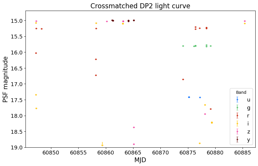
../../_images/tutorials_pre_executed_full_dp2_crossmatches_30_0.png

[18]:

band_colors = {
    "u": "#0c71ff",
    "g": "#49be61",
    "r": "#c61c00",
    "i": "#ffc200",
    "z": "#f341a2",
    "y": "#5d0000",
}

mag_cut = 19.0  # faint-end cutoff (inverted magnitude axis)

fig, ax = plt.subplots(figsize=(10, 6))

# One error-bar series per band, colored by filter, with capped error bars
for band in band_colors:
    grp = lc[lc["band"] == band]
    if len(grp) == 0:
        continue
    ax.errorbar(
        grp["midpointMjdTai"],
        grp["psfMag"],
        yerr=grp["psfMagErr"],
        fmt="o",
        markersize=3,
        alpha=0.6,
        ls="none",
        capsize=2,
        color=band_colors[band],
        label=band,
    )

# Inverted axis, cut off at the faint end (mag 19); brighter objects sit higher
top = lc.loc[lc["psfMag"] <= mag_cut, "psfMag"].min() - 0.3
ax.set_ylim(mag_cut, top)

# Points fainter than the cutoff fall off the bottom: mark each epoch with a
# down-arrow colored by its band
for _, row in lc[lc["psfMag"] > mag_cut].iterrows():
    ax.annotate(
        r"$\downarrow$",
        xy=(row["midpointMjdTai"], mag_cut),
        ha="center",
        va="bottom",  # bottom of the glyph aligns with the axis
        color=band_colors[row["band"]],
        fontsize=14,
        annotation_clip=False,
    )

ax.set_xlabel("MJD")
ax.set_ylabel("PSF magnitude")
ax.set_title("Crossmatched DP2 light curve")
ax.legend(title="Band")
plt.show()

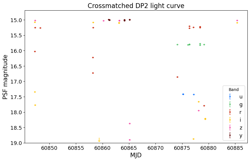
../../_images/tutorials_pre_executed_full_dp2_crossmatches_31_0.png

Summary#

With an RSP-sized environment, it’s possible to do large crossmatches between DP2 and other large HATS catalogs, as long as you are mindful of the columns being loaded and the Dask Client setup you are specifying for computation. Note how much the computational approach needed to change just by including lightcurves from “objectForcedSource”. Being aware of the computational weight of your workflows is it’s own learning curve, even as LSDB tries to assist as much as it can with this.

If you’re looking for more tips on doing large scale workflows, consult the LSDB documentation.

About#

Author(s):Doug Branton

Last run: July 27, 2026

If you use lsdb for published research, please cite following instructions.